Calculating MQO Statistics • mqor

library(mqor)

Calculating statistics is the most important part of the mqor package; all other functionality flows from this point.

For mathematical descriptions of all of the statistical indicators, see the definitions article.

Model Evaluation Parameters

There are four parameters required for most model evaluation functions in mqor.

rv - Reference value. A numeric value, used to define the relationship between measurement uncertainty and concentration level, for each pollutant and time aggregation. rv is expressed in the same units as the concentration of the pollutant.
u_rv - Maximum accepted relative measurement uncertainty. A numeric value, expressed as a percent (0.1 is equivalent to 10%).
a - The alpha parameter. Fraction of the maximum accepted measurement uncertainty that is not proportional to the concentration, ranging between 0 and 1. It is pollutant and measurement-type specific.
b - The beta parameter. Ratio between the maximum accepted modelling and measurement uncertainties for short- and long-term averages. It is pollutant and measurement-type specific, and it determines the stringency of the MQO. The stringency factor β corresponds to the maximum ratio of uncertainty of modelling applications as specified in the AAQD.

mqor attempts to select appropriate default values from the CEN working document, but users can construct their own parameter sets if they wish. There are a number of ways to achieve this in mqor:

mqo_params() allow users to conveniently create a parameter set using their own values.
mqo_params_default() allows users to obtain ‘default’ values for different pollutants, time periods, and monitoring types (indicative versus fixed).
Users can construct their own object (either R list or data.frame) as long as it has names rv, u_rv, a and b which can be index by mqor functions.

The default parameters which mqo_params_default() samples from are available to the users in the default_params dataset.

default_params

pollutant	term	time	status	rv_unit	rv	u_rv	a	b	type
no2	short	hourly	normative	ug/m3	200.0	0.15	0.200	3.20	fixed
o3	short	max daily 8hr mean	normative	ug/m3	120.0	0.15	0.400	2.20	fixed
pm10	short	daily	normative	ug/m3	45.0	0.25	0.350	2.20	fixed
pm2.5	short	daily	normative	ug/m3	25.0	0.25	0.600	2.50	fixed
no2	short	hourly	normative	ug/m3	200.0	0.25	0.900	1.92	indicative
o3	short	max daily 8hr mean	normative	ug/m3	120.0	0.25	0.800	1.32	indicative
pm10	short	daily	normative	ug/m3	45.0	0.50	0.850	1.10	indicative
pm2.5	short	daily	normative	ug/m3	25.0	0.35	0.830	1.79	indicative
no2	long	annual	normative	ug/m3	20.0	0.30	0.975	1.40	fixed
o3	long	seasonal	normative	ug/m3	60.0	0.15	0.400	1.70	fixed
pm10	long	annual	normative	ug/m3	20.0	0.20	0.600	1.30	fixed
pm2.5	long	annual	normative	ug/m3	10.0	0.30	0.800	1.70	fixed
no2	long	annual	normative	ug/m3	20.0	0.40	0.975	1.05	indicative
o3	long	seasonal	normative	ug/m3	60.0	0.25	0.800	1.02	indicative
pm10	long	annual	normative	ug/m3	20.0	0.30	0.800	0.87	indicative
pm2.5	long	annual	normative	ug/m3	10.0	0.40	0.900	1.28	indicative
no2	short	daily	informative	ug/m3	50.0	0.15	0.800	3.20	fixed
no2	short	daily	informative	ug/m3	50.0	0.25	0.940	1.92	indicative
so2	short	daily	informative	ug/m3	50.0	0.15	0.600	3.20	fixed
so2	short	daily	informative	ug/m3	50.0	0.25	0.920	1.92	indicative
so2	short	hourly	informative	ug/m3	350.0	0.15	0.150	3.20	fixed
so2	short	hourly	informative	ug/m3	350.0	0.25	0.930	1.92	indicative
co	short	daily	informative	mg/m3	4.0	0.15	0.900	3.20	fixed
co	short	daily	informative	mg/m3	4.0	0.25	0.950	1.92	indicative
co	short	max daily 8hr mean	informative	mg/m3	10.0	0.10	0.500	4.90	fixed
co	short	max daily 8hr mean	informative	mg/m3	10.0	0.20	0.950	2.45	indicative
so2	long	annual	informative	ug/m3	20.0	0.30	NA	1.40	fixed
so2	long	annual	informative	ug/m3	20.0	NA	NA	1.05	indicative
benzene	long	annual	informative	ug/m3	3.4	0.25	0.550	1.70	fixed
benzene	long	annual	informative	ug/m3	3.4	0.35	0.550	1.21	indicative
lead	long	annual	informative	ug/m3	0.5	0.25	0.500	1.70	fixed
lead	long	annual	informative	ug/m3	0.5	NA	NA	NA	indicative
arsenic	long	annual	informative	ng/m3	6.0	0.40	0.300	1.10	fixed
arsenic	long	annual	informative	ng/m3	6.0	NA	NA	NA	indicative
cadmium	long	annual	informative	ng/m3	5.0	0.40	0.300	1.10	fixed
cadmium	long	annual	informative	ng/m3	5.0	NA	NA	NA	indicative
nickel	long	annual	informative	ng/m3	20.0	0.40	0.300	1.10	fixed
nickel	long	annual	informative	ng/m3	20.0	NA	NA	NA	indicative
bap	long	annual	informative	ng/m3	1.0	0.50	NA	1.10	fixed
bap	long	annual	informative	ng/m3	1.0	NA	NA	NA	indicative

Creating Statistical Summaries

The summarise_mqo_stats() function is a shorthand for applying all of MQO statistic functions on an R data frame, and will be of the most use to most users. This function provides a complete set of statistics; ‘per site’ (e.g., the MQI) and an overall summary of the data (e.g., the 90th percentile MQI), plus ‘per type’ for long-term data. The exact structure of this output varies with the data ‘term’, but both objects contain a $inputs item which contains the term, pollutant, params_fixed and params_indicative (the latter two coerced into data.frames) used in the calculations.

Note that this function will attempt to guess the ‘term’ of the data, based on whether each site is represented by one row of the dataframe (‘long-term’ data) or by multiple rows (‘short-term’ data). If the function assumes incorrectly, users are free to specify "short" or "long" by using the term argument.

As demo_shortterm and demo_longterm are both PM10 datasets, and PM10 is included in default_params, we don’t need to specify fixed or indicative parameters in these examples; the function automatically attempts to use mqo_params_default() to choose appropriate parameters.

Long Term Statistics

stats_long <- summarise_mqo_stats(demo_longterm, pollutant = "PM10")
#> ! term assumed to be 'long'.
#> ℹ If this is incorrect, please specify the data's term using the term argument.

stats_long
#> 
#> ── mqor Statistics Set ─────────────────────────────────────────────────────────
#> ✔ MQO Passed
#> Pollutant: PM10
#> Term: long
#> 
#> ── Objects ──
#> 
#> • x$summary (1 row)
#> • x$by_type (1 row)
#> • x$by_site (15 rows)
#> • x$inputs

Overall Summary ($summary)
- bias: Bias.
- rmse: Root Mean Square Error.
- r: Correlation coefficient.
- sd_obs, sd_mod: Standard deviation in observed and modelled values.
- rmsu: Root Mean Square Uncertainty.
- mqi_90: The 90th percentile of the Model Quality Indicator.
- mqo: A boolean value as to whether the Model Quality Objective has been met (i.e., if mqi_90 <= 1).
By Type ($by_type)
- type: One of "fixed" or "indicative".
- si_rmse, si_bias, si_cor, si_sd: Complementary ‘Spatial Performance Indicators’ which combine other indicators with the beta coefficient and rmsu.
By Site ($by_site)
- site: The site identifier; could be a name, an ID, an abbreviation, etc.
- type: One of "fixed" or "indicative".
- param: The pollutant or meteorological parameter being assessed.
- obs, mod: The observed or modelled concentration from the input data.
- uncer: The Maximum Accepted Measurement Uncertainty.
- ar_low, ar_up: The ‘acceptability range’ of the monitored data; used in plot_comparison_bars().
- mqi: The model quality indicator; used to assess the network against the model quality objective.

Short Term Statistics

stats_short <- summarise_mqo_stats(demo_shortterm, pollutant = "PM10")
#> ! term assumed to be 'short'.
#> ℹ If this is incorrect, please specify the data's term using the term argument.

stats_short
#> 
#> ── mqor Statistics Set ─────────────────────────────────────────────────────────
#> ✔ MQO Passed
#> Pollutant: PM10
#> Term: short
#> 
#> ── Objects ──
#> 
#> • x$summary (1 row)
#> • x$by_site (15 rows)
#> • x$inputs

Overall Summary ($summary)
- mqi_90: The 90th percentile of the Model Quality Indicator.
- mqo: A boolean value as to whether the Model Quality Objective has been met (i.e., if mqi_90 <= 1).
- ti_bias_90, ti_cor_90, ti_sd_90: The 90th percentile of the complementary ‘Temporal Performance Indicators’ which combine other indicators with the beta coefficient and rmsu.
By Site ($by_site)
- site: The site identifier; could be a name, an ID, an abbreviation, etc.
- type: One of "fixed" or "indicative".
- mean_obs, mean_mod: The mean observed and modelled concentrations for each site.
- bias: Bias.
- rmse: Root Mean Square Error.
- rmsu: Root Mean Square Uncertainty.
- rmsu_star: The rmsu combined with the beta coefficient; used in plot_comparison_bars()
- r: Correlation coefficient.
- sd_obs, sd_mod: Standard deviation in observed and modelled values.
- crmse: Centred Root Mean Square Error
- mqi: The model quality indicator; used to assess the network against the model quality objective.

Dynamic Table

It is possible to create a dynamic, sortable table from statistics sets using tabulate_mqo_stats(). This may be easier to examine than the ‘raw’ R list output.

tabulate_mqo_stats(stats_short)

tabulate_mqo_stats(stats_long)

Calculating Individual Statistics

mqor also has many functions for calculating MQO-related statistics. These all apply to vectors, making them ideal for use in dplyr functions.

param_set <- 
  mqo_params_default(
      term = "long",
      type = "fixed",
      pollutant = "pm10"
    )

# apply to R vector
vec_mqi(
  obs = 90,
  mod = 50,
  term = "long",
  params = param_set
)
#> [1] 1.670597

# use with dplyr
dplyr::summarise(
  demo_longterm,
  mqi = vec_mqi(
    obs,
    mod,
    term = "long",
    params = param_set
  ),
  .by = site
)
#> # A tibble: 15 × 2
#>    site    mqi
#>    <chr> <dbl>
#>  1 S1    0.833
#>  2 S2    0.342
#>  3 S3    0.411
#>  4 S4    0    
#>  5 S5    0.518
#>  6 S6    0.355
#>  7 S7    0.525
#>  8 S8    0.158
#>  9 S9    0.171
#> 10 S10   0.261
#> 11 S11   1.72 
#> 12 S12   0.791
#> 13 S13   0.732
#> 14 S14   0.890
#> 15 S15   0.443

Tuning Statistics

Being able to flexibly calculate statistics allows users to experiment with parameters via iteration and extracting relevant MQI data. As a simple example, the below code works out the range of mod values which pass the MQO when obs = 75.

opts <- 0:100

id <-
  purrr::map_vec(
    .x = 0:100,
    .f = \(x)
    vec_mqi(
      obs = 75,
      mod = x,
      term = "long",
      params = param_set
    )
  )

range(opts[which(id <= 1)])
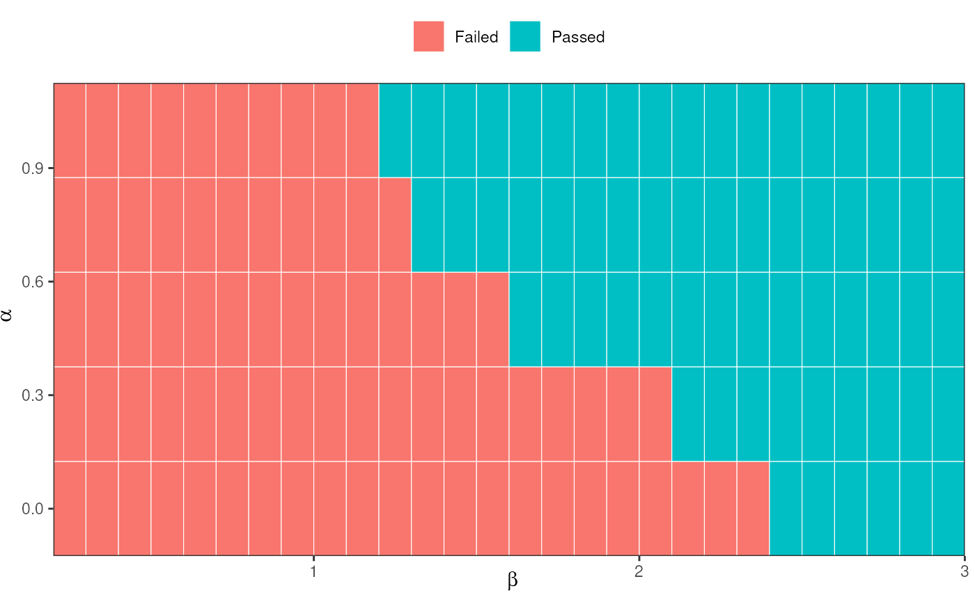
#> [1] 55 95

The example below is more complex, using summarise_mqo_stats(). In this case, the user is varying the ‘alpha’ and ‘beta’ coefficients and examining their influence on the MQO[90th].

library(ggplot2)

vary <-
  expand.grid(
    a = seq(0, 1, 0.25),
    b = seq(0.25, 3, 0.1)
  ) |>
  purrr::pmap(
    .f = function(a, b) {
      params <- mqo_params(
        rv = 45,
        u_rv = 0.25,
        a = a,
        b = b
      )

      out <- summarise_mqo_stats(
        demo_shortterm,
        pollutant = "PM10",
        term = "short",
        params_fixed = params, 
        table = "summary"
      )

      data.frame(mqi90 = out$mqi_90, mqo = out$mqo, beta = b, alpha = a)
    }
  ) |>
  dplyr::bind_rows()

ggplot(vary, aes(x = beta, y = alpha, fill = ifelse(mqo, "Passed", "Failed"))) +
  geom_tile(color = "white") +
  theme_bw() +
  labs(x = expression(beta), y = expression(alpha), fill = NULL) +
  theme(legend.position = "top") +
  coord_cartesian(expand = FALSE)

A ggplot2.