An Introduction to {mqor} • mqor

library(mqor)

Overview

The mqor package implements the methodology contained in “Ambient Air — Definition and use of modelling quality objectives for air quality assessment”. This ‘getting started’ guide provides a basic overview of using mqor for model evaluation.

The below flowchart shows how data moves through mqor.

A flowchart showing how data moves through mqor

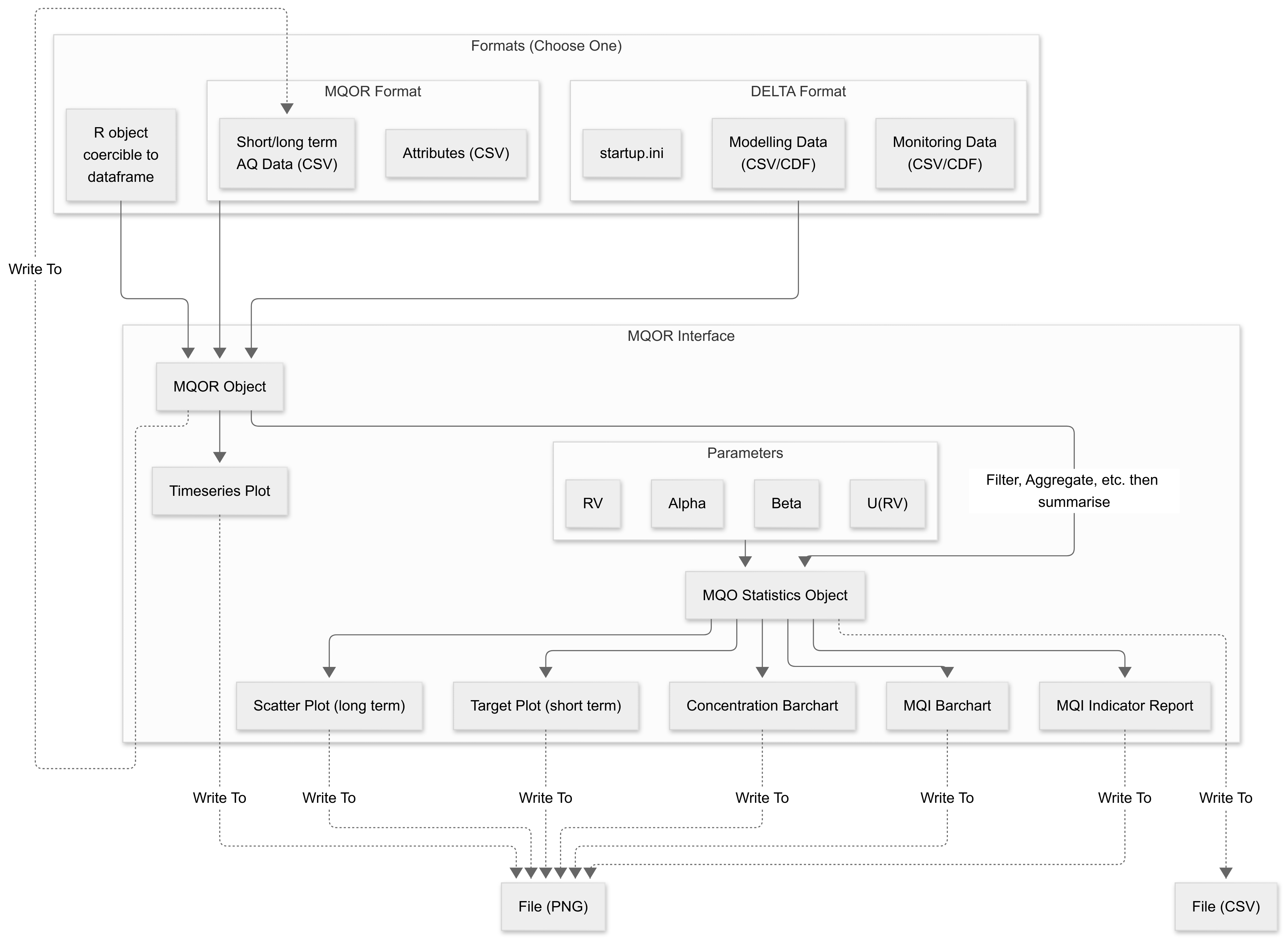
Users can provide data from one of three sources:

Input files expected by the DELTA tool. For the monitoring and measurement data, this can either be a CDF or a directory of delimited files. The startup.ini is also additionally required, formatted as expected by the DELTA tool. No other DELTA config files are required.
An alternative “simplified” data format, originally developed alongside mqor during its inception project.
Any kind of R object which the user can coerce into a data.frame (or tibble). It is up to the user to ensure that this data is in an appropriate.

The MQO in practice

Introduction

This section reproduces ‘The MQO in practice’ annex of the MQO technical specification. More in-depth descriptions of these steps are found in the articles section on this package website. The examples in this annex are for a network of fixed sampling points, and are made available through mqor as demo_shortterm and demo_longterm. For convenience, long-term MQO is first addressed, short-term MQO afterwards. Any statistics that are not defined here should be presented in the mqor definitions article.

Long-term MQO

The figures in this section illustrate the application of the long-term MQI calculation and MQO evaluation for a dataset of 15 fixed measurement sampling points.

Step A (long) – Comparison of modelled and measured values

We should first calculate the necessary statistical indicators on the data. By default, this function works out whether the input data is long- or short-term, and attempts to look up the default values defined by the CEN technical specification. Values for $\beta_{long}$ (1.30), $RV_{long}$ (20), $U_{Or}(RV_{long})$ (0.2) and $\alpha_{long}$ (0.6) are the defaults for long-term PM10 found within the default_params dataset. Under the hood, these are obtained using mqo_params_default(term = "long", type = "fixed", pollutant = "PM10"), which a user could choose to provide themselves.

# let mqor work out the default values
long_stats <- summarise_mqo_stats(demo_longterm, pollutant = "PM10")
#> ! term assumed to be 'long'.
#> ℹ If this is incorrect, please specify the data's term using the term argument.

# OR provide them manually
# long_stats <-
#   summarise_mqo_stats(
#     demo_longterm,
#     pollutant = "PM10",
#     params_fixed = mqo_params(rv = 20, u_rv = 0.2, a = 0.6, b = 1.3)
#   )

The bar chart below shows the comparison of annual averaged measured PM10 (grey bars) and modelled values (black bars).

To illustrate whether the modelled values for each sampling point meet the $MQI_{long} \leq 1$ , we introduce the concept of the performance acceptability range (AR), the upper and lower bounds of which are defined using the equation below. Modelled values meeting the $MQI_{long} \leq 1$ for a particular sampling point are within the lower and upper bounds of the AR for the measured values at that sampling point.

$AR = \bar{O} \pm \sqrt{1 + \beta^2_{long}} U_O(\bar{O})$

As an example, for the sampling point S1, AR would be calculated as: $AR = 34 \pm \sqrt{1 + 1.3^2} \cdot6$ leading to values of $AR_{low}$ and $AR_{up}$ of 24.56 and 44.24, respectively. In this calculation, the below formula has been used to derive $U_{O}(\bar{O})$ as:

$U_O(34.4) = 0.2 \cdot \sqrt{(1-0.6^2)\cdot34.4^2+0.6^2\cdot20^2} = 6.00$

The AR range is displayed as a vertical line on top of the measured value. The values of the lower and upper bounds of the AR range are indicated in the table below for each sampling point. Modelled values meeting the $MQI_{long} \leq 1$ for a particular sampling point are within the lower and upper bounds of the AR for the measured values at that sampling point.

The plot_comparison_bars() function creates this plot. It only requires the statistics object that has already been created.

plot_comparison_bars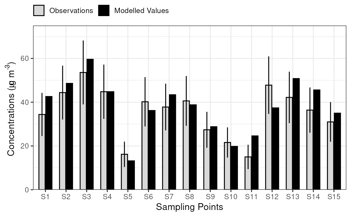(long_stats)

Application of the long-term MQI for an arbitrary sample dataset of 15 sampling points (S1 to S15) for PM10.

Numerical values of the parameters associated with the long-term dataset for PM10.
	S1	S2	S3	S4	S5	S6	S7	S8	S9	S10	S11	S12	S13	S14	S15
О̄	34.40	44.40	53.60	44.8	16.20	40.20	37.80	40.60	27.40	21.60	15.00	47.80	42.20	36.40	31.00
M̄	42.60	48.60	59.60	44.8	13.20	36.20	43.40	38.80	28.80	19.80	24.60	37.40	50.80	45.60	35.00
AR (low)	24.55	32.10	38.99	32.4	10.41	28.94	27.13	29.24	19.20	14.70	9.43	34.65	30.45	26.07	21.96
AR (up)	44.25	56.70	68.21	57.2	21.99	51.46	48.47	51.96	35.60	28.50	20.57	60.95	53.95	46.73	40.04
MQI (long)	0.83	0.34	0.41	0.0	0.52	0.36	0.52	0.16	0.17	0.26	1.72	0.79	0.73	0.89	0.44

Step B (long) – Analysis of the MQI/MQO

The $MQI_{long}$ of each sampling point are calculated and are then sorted in ascending order. The below formulae serve to calculate the 90th percentile MQI as follows:

$N_{90th} = floor(0.9N_s)$

$D = 0.9N_s-N_{90th}$

$MQI_{long,90th} = MQI_{long}(N_{90th}) + (MQI_{long}(N_{90th}+1)-MQI_{long}(N_{90th})) \cdot D$

plot_mqi_bars(long_stats)

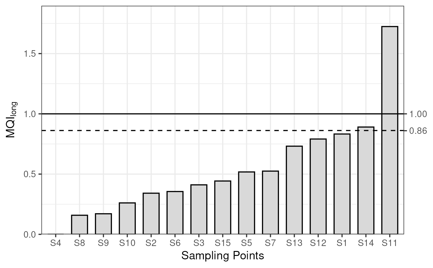
Application of the long-term MQI(long), MQI(long,90th) and MQO(long) for an arbitrary sample dataset of 15 sampling points for PM10.

The 90th percentile $MQI_{long}$ is then compared to unity to assess fulfilment of the $MQO_{long}$ .

For the long-term $MQO:MQI_{long,90th} = 0.86 \leq 1.00$

In our example, the modelling application fulfils the $MQO_{long}$ and is suitable for assessment. Nevertheless, fulfilling the $MQO_{long}$ does not prevent further investigation based on situations for individual sampling points where the $MQI_{long}$ is large, to enhance the quality of the modelling application (e.g. sampling point S11 in our example). When relevant, a similar approach applies to the calculation of the short-term $MQI_{short}$ .

Step C (long) – Scatter diagram of the MQI/MQO

A scatter diagram, that includes information on the acceptability range is used as the main visualisation to summarise the modelling performance validation with the $MQI$ and $MQO$ .

plot_mqi_scatter(stats_long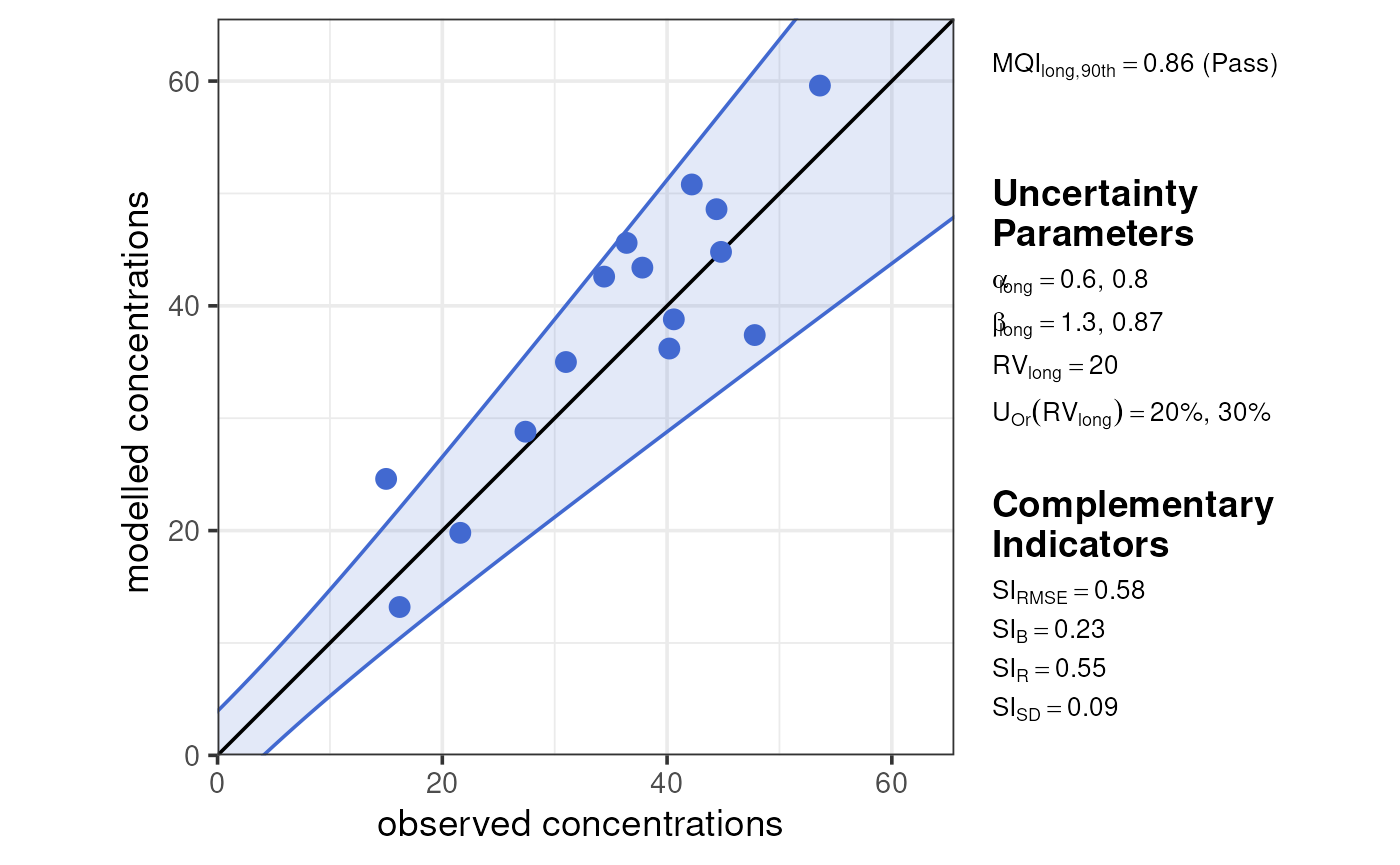term = long_stats)

In the scatter diagram, the value of the $MQI_{long,90th}$ as well as an indication on whether the MQO is fulfilled or not (pass or fail) is displayed. The value of the uncertainty parameters $\alpha_{long}$ , $\beta_{long}$ , $U_{Or}(RV_{long})$ and $RV_long$ used to produce the diagram are listed on the side of the figure. The values obtained for the complementary spatial performance indicators (see: statistical indicator definitions) are also reported together with the scatter diagram.

Short Term MQO

Calculation of MQI (short)

The short-term MQO is based on the $MQI_{short}$ .

This section illustrates the application of the MQI short for 15 fixed sampling points (S), for a timeseries of observed (O (t)) and modelled (M(t)) values including 5 timesteps. In this example the values represent 5 daily values of PM10. In practice the data is required to cover an entire year within appropriate data coverage constraints.

At first the root mean square error (RMSE) of modelled PM10 values shall be calculated (grey bars). Following this the product of the root mean square of the maximum measurement uncertainty ( $RMSU_{O}$ ) and the stringency factor ( $\sqrt{1+\beta_{short}^2}$ ) is to be calculated (black bars).

Values for $\beta_{short}$ (2.2), $RV_{short}$ (45), $U_{Or}$ ( $RV_{short}$ ) (0.25) and $\alpha_{short}$ (0.35) for PM10.

mqor also provides the demo_shorterm dataset for demonstration purposes.

Step A (short) – Comparison of modelled and measured root mean squares

This bar chart shows the comparison of the root mean square error (RMSE) in modelled PM10 values (grey bars) with the product of the root mean square of the maximum measurement uncertainty ( $RMSU_{O}$ ) and the stringency factor ( $\sqrt{1+\beta_{short}^2}$ ) (black bars). Since $MQI_{short}$ for a time series at one sampling point is expressed as $MQI_{short}=RMSE~/ \sqrt{1+\beta_{short}^2}\cdot RMSU_{O}$ . It is necessary for the grey bars to be lower than or the same height as the black ones for the modelled PM10 values to fulfil $MQI_{short} \leq 1$ . This is the case for all sampling points except S9 and S11.

As an example, for sampling point S1, calculations of the $RMSE$ and $RMSU_{O}$ lead to:

$RMSE = \sqrt{\frac{1}{N_t}\sum_{t=1}^{N_t}{(O(t)-M(t))^2}} = \sqrt{\frac{1}{5}[(24-48)^2+(35-47)^2+(44-39)^2+(38-37)^2+(31-42)^2]}=13.2$

$RMSU_{O} = U_{Or}(RV_{short})\sqrt{(1-\alpha^2_{short})(\bar{O}^2+\sigma^2_o)+\alpha^2_{short}RV^2_{short}}=\sqrt{(1-0.35^2)(34.4^2+6.71^2)+0.35^2\cdot45^2}=9.10$

The product of the root mean square of the maximum measurement uncertainty ( $RMSU_{O}$ ) by the stringency factor ( $\sqrt{1+\beta_{short}^2}$ ) is equal to 22.0.

The below formula is used to calculate the $MQI_{short}$ of the timeseries at sampling point S1 for PM10 leading to $MQI_{short}=0.60$ .

$MQI_{short} = \frac{RMSE}{\sqrt{1+\beta_{short}^2}\cdot RMSU_{O}}$

short_stats <- summarise_mqo_stats(demo_shortterm, pollutant = "PM10")
#> ! term assumed to be 'short'.
#> ℹ If this is incorrect, please specify the data's term using the term argument.

plot_comparison_bars(s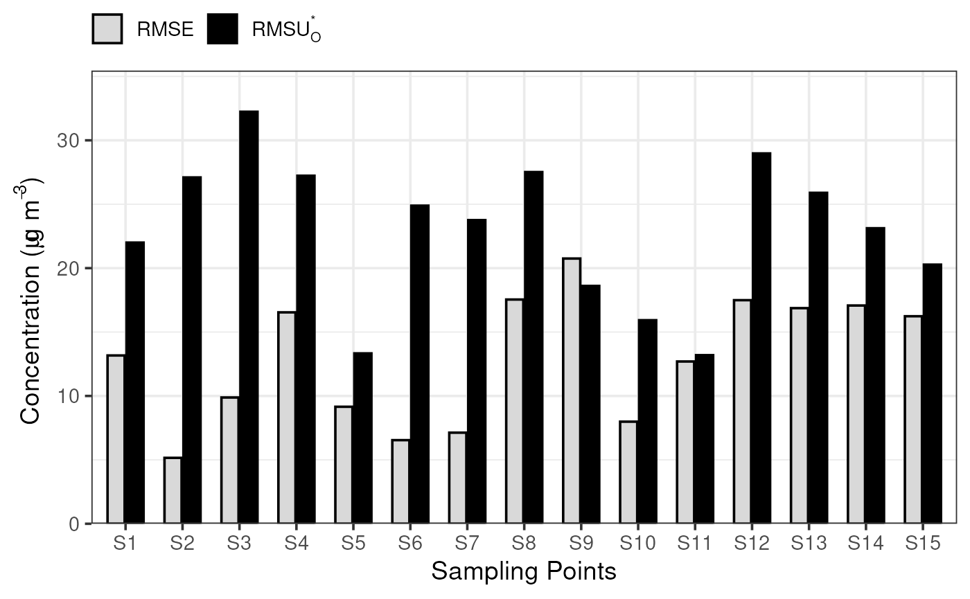hort_stats)

Application of the short-term MQIshort for an arbitrary sample dataset of 15 sampling points (S1 to S15, each composed of 5 time-steps (t=1 to 5)) for PM10

Numerical values of the parameters associated with the short-term dataset for PM10
	S1	S2	S3	S4	S5	S6	S7	S8	S9	S10	S11	S12	S13	S14	S15
M(1)	48	36	50	23	21	30	34	30	0	13	12	37	48	50	37
M(2)	47	49	61	42	21	36	56	47	80	36	27	24	59	40	37
M(3)	39	61	70	50	12	43	47	52	21	22	34	47	49	48	37
M(4)	37	53	66	59	4	39	42	36	24	17	32	44	36	55	17
M(5)	42	44	51	50	8	33	38	29	19	11	18	35	62	35	47
O(1)	24	37	37	50	12	33	31	18	22	12	15	46	46	38	33
O(2)	35	45	51	51	16	50	44	80	40	24	5	54	38	38	28
O(3)	44	53	57	44	21	43	48	35	29	29	22	46	44	38	33
O(4)	38	49	65	38	18	39	36	37	25	27	20	36	49	22	40
O(5)	31	38	58	41	14	36	30	33	21	16	13	57	34	46	21
RMSE	13.2	5.2	9.9	16.5	9.2	6.5	7.1	17.5	20.8	8	12.7	17.5	16.9	17.1	16.2
RMSU(O)	9.1	11.2	13.3	11.3	5.5	10.3	9.8	11.4	7.7	6.6	5.5	12	10.7	9.6	8.4
RMSU(O)*	22	27.1	32.2	27.2	13.3	24.9	23.8	27.5	18.6	15.9	13.2	29	25.9	23.1	20.3
MQI (short)	0.6	0.19	0.31	0.61	0.69	0.26	0.3	0.64	1.12	0.5	0.96	0.6	0.65	0.74	0.8

Step B (short) – Analysis of the MQI/MQO

The below formula is used to calculate the $MQI_{short}$ of each sampling point that are then sorted. The 90th percentile MQI is calculated as follows:

$N_{90th} = floor(0.9N_s) = floor(13.5) = 13$

$D = 0.9N_s-N_{90th} = 0.9 \cdot 15 - 13 = 0.5$

$MQI_{short,90th} = MQI_{short}(N_{90th}) + (MQI_{short}(N_{90th}+1)-MQI_{short}(N_{90th})) \cdot D = 0.801 + (0.962 - 0.801) \cdot 0.5 = 0.88$

plot_mqi_bars(short_stats)

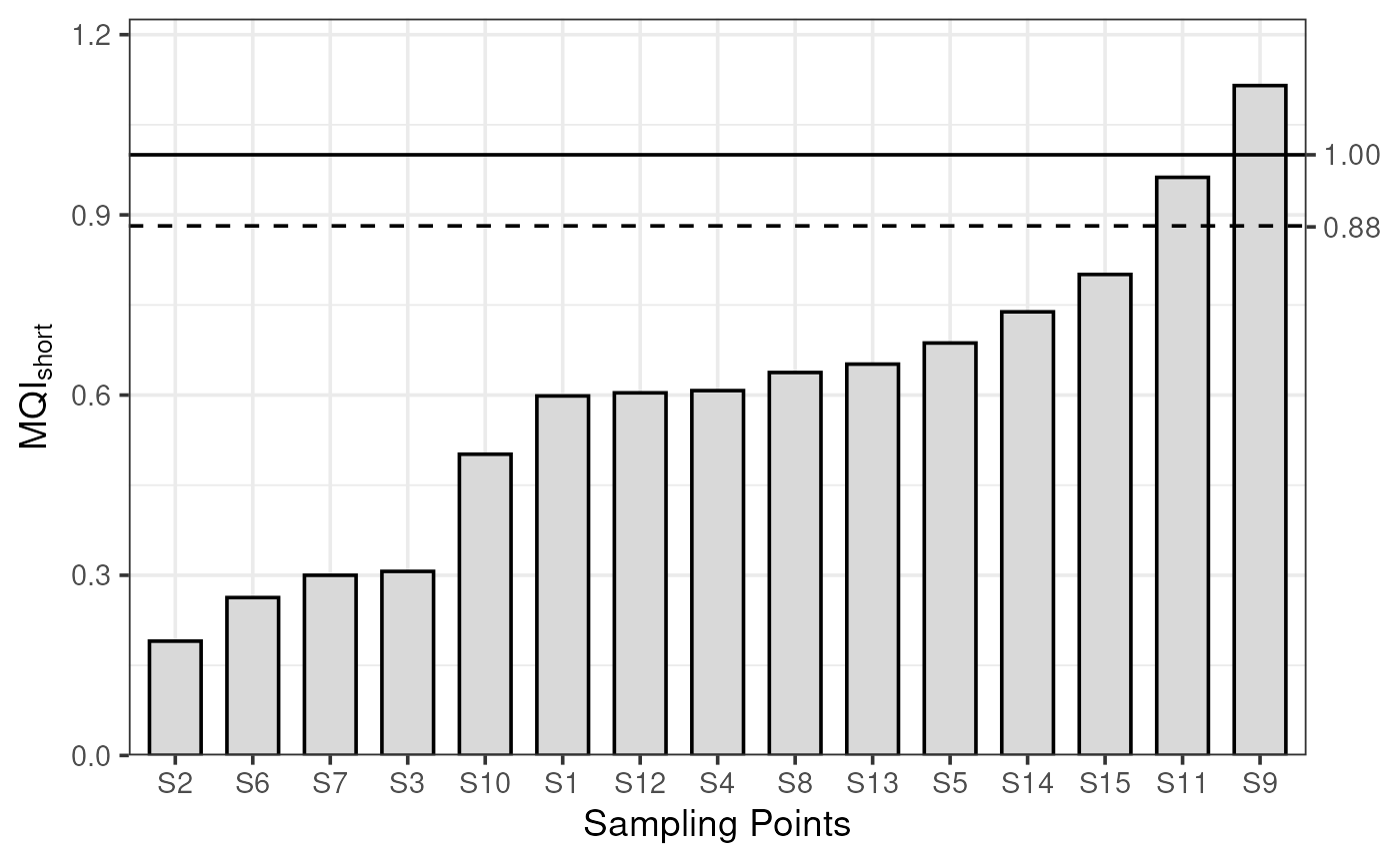
Application of the short—term MQIshort, MQIshort,90th and MQOshort for an arbitrary sample dataset of 15 sampling points for PM10

The 90th percentile $MQI_{short}$ is then compared to unity to assess fulfilment of the $MQO_{short}$ .

$MQO_{short}:MQI_{short,90th} = 0.88 \leq 1.00$ In our example, the modelling application fulfils the $MQO_{short}$ and is suitable for assessment. Nevertheless, fulfilling the $MQO_{short}$ does not prevent further investigation based on situations for individual sampling points where the $MQI_{short}$ is large, to enhance the quality of the modelling application (e.g., sampling points S9 and S11 in our example).

Step C (short) – Target diagram of the MQI/MQO

The uncertainty normalised target diagram is used as main diagram for visualisation of the $MQI_{short}$ and $MQO_{short}$ . The $MQI_{short}$ for a given sampling point represents the distance between the origin and the location of the sampling point symbols.

In the target diagram the abscissa and ordinate correspond to $TI_{CRMSE}$ and $TI_{Bias}$ and the radius is equal to the $MQI_{short}$ (see: statistical indicator definitions). The shaded area on the Target diagram identifies the area of fulfilment of the $MQI_{short}$ . 90% of the available sampling points should have their symbols located within this shaded area.

The choice of sign for $TI_{CRMSE}$ (positive or negative) provides information on whether it is dominated by correlation or by standard deviation. The ratio of $TI_{R}$ and $TI_{\sigma}$ serves as basis to decide on which side of the Target diagram the point is located:

$\frac{|TI_{\sigma}|}{TI_{R}} = \frac{|\sigma_M-\sigma_O|}{\sqrt{2\sigma_{O}\sigma_{M}(1-R)}} \begin{cases}>1 : \sigma~dominates~R : right \\ <1 : R~dominates~\sigma : left\end{cases}$

For ratios larger than 1 the $\sigma$ error dominates and the sampling point is represented on the right abscissa section, whereas for values smaller than 1 the sampling point is represented on the left abscissa section.

The MQI associated to the 90th percentile worst sampling point is calculated and indicated in the upper part of the diagram, both for short- and long-term averages applications, together with a pass/fail information. Both the $MQI_{short,90th}$ and $MQI_{long,90th}$ should be less or equal to unity.

plot_mqi_scatter(stats_shortterm = short_stats, stats_long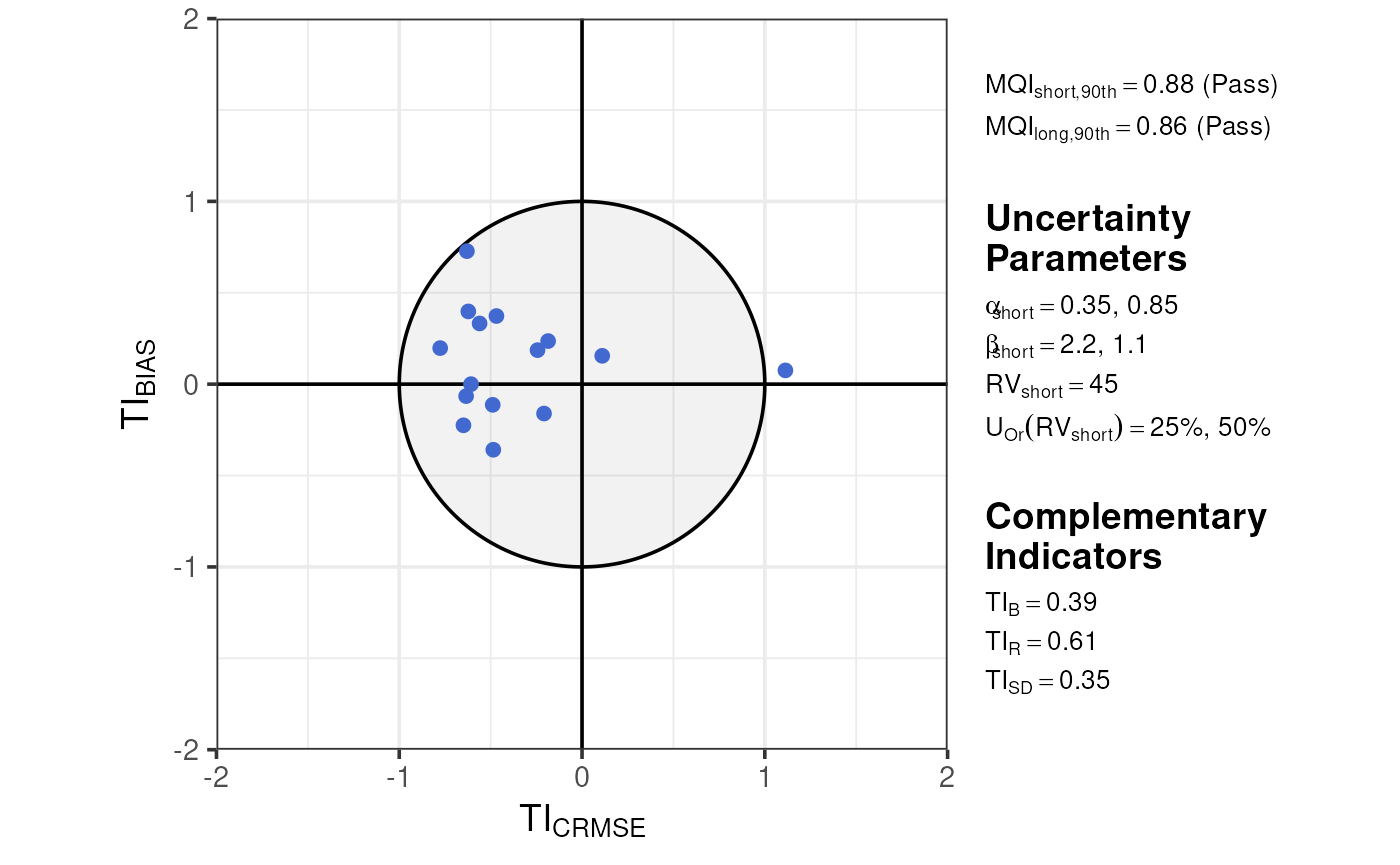term = long_stats)

In the target diagram, the value of both the $MQI_{short,90th}$ and the $MQI_{long,90th}$ as well as an indication on whether these MQO are fulfilled or not (pass or fail) are displayed. The value of the short-term uncertainty parameters used to produce the diagram are listed on the side. The values obtained for the complementary temporal performance indicators are also be reported together with the target diagram.

Next Steps

mqor has many other features than those outlined here. Plots can be customised, and interactive plots can be generated. There are several data utilities to help construct daily average values or rolling averages. The tabulate_mqo_stats() and plot_mqi_report() can be used to create attractive alternative visualisations fpr the MQI/MQO.

To explore mqor further, you may now wish to:

Explore some of the themes above (importing data, calculating statistics, plotting data) by working your way through the package articles.
View the full breadth of mqor functionality, including how to access alternative sample datasets, in the function reference page.
Have a look at some self-contained code ‘recipes’ for use in an interactive R session.
Use mqor’s interactive interface, described in the Shiny Interface Guide.