Shiny Interface

While using mqor interactively will give you the greatest flexibility over calculating model performance, you may not be comfortable running code. mqor contains the function launch_app() which launches a web interface in your browser to allow you to use mqor functionality without needing to write any R scripts.

mqor::launch_app()

This application should launch in your web browser. While effort has been made to ensure that it appears nicely on your screen, if you have an unusual screen size or dimensions you may wish to zoom in and out on your browser for a more comfortable experience.

First Screen: Data Upload

On launching the app you will be met with an empty map and a sidebar with several options. The first drop-down option defines the data input format; either the “MQOR” format (that an ‘interactive’ user would read with read_mqor()) or the “DELTA” format (that would be read with read_delta_data_delim(), read_delta_yearly_file(), etc.).

“DEMO” can also be selected, which loads a very simple dataset to help explore the functionality of the rest of the application if you have no data prepared.

Regardless of the data format you choose, once you have provided all of your files clicking the ‘Upload Data’ button will begin reading them into R. Once this process has finished, the monitoring map will update and the “MQO Explorer” tab will be unlocked.

MQOR Format

If using the “MQOR” format, you must upload an ‘attributes’ CSV file and any number of files for short- and long-term data. You may provide both short- and long-term data, only long-term data, or only short-term data. If only short-term data is provided, an annual mean of the given data will be used to calculate the long-term data.

DELTA Format

The DELTA format has many more combinations of formats than the MQOR format. You may need to provide up to 5 files; short-term monitoring, short-term modelling, long-term monitoring, long-term monitoring, and the ‘startup.ini’ metadata file. For the first three of these, radial buttons allows you to switch between different formats - multiple CSVs vs one CDF file for the short-term data, and a single vs multiple CSVs for the long-term monitoring data.

DELTA tool input data does not include any flags as to whether data are fixed or indicative. You must therefore also state whether you wish to treat your DELTA-formatted data as fixed or indicative. For finer control, consider running mqor interactively or providing data in the MQOR format.

Second Screen: MQO Explorer

Once data has been selected, you may select the “MQO Explorer” tab in the navigation bar at the top of the screen. Initially, the main panel of the dashboard will be empty; you must first select and filter data using the sidebar.

Parameter Selection

The first filtering step is to select your desired pollutant and year. This applies globally to all short- and long-term data.

Attribute Filtering

Data can also be filtered by monitoring station attributes (e.g., site type, region, and so on). The option to filter by fixed or indicative monitoring is always present. As there are potentially many other attributes - and, in the case of DELTA formatted data, any arbitrary number of other attributes - you must first select the attributes you would like to filter on (if any) which will then spawn additional check boxes for filtering. Note that any category which contains a constant value will not be presented as an option; if all of your monitoring stations are urban sites, then you will not be presented with the option to filter on urbanity.

Attribute filtering applies to both short- and long-term data.

Short Term Data Handling

There a few options for handling short-term data:

• Resolution & Data Capture: Here you can define whether your short-term data is hourly, daily or ‘other’ (which disables data capture checks). If either of ‘hourly’ or ‘daily’, the input data will be padded to a complete time series and then filtered to ensure data capture thresholds are met. Note that, if you wish to use ‘temporal filtering’ (below) it may be appropriate to lower your data capture threshold. Note that long-term data (including that provided by the user) will be filtered so the same sites are present in both datasets.

• Temporal Filtering: Short-term data can be filtered by the month of the year, day of the week, and hour of the day. Through combining these options, you are able to flexibly filter your data for specific seasons, daytime vs nighttime, and so on.

• Data Processing: Short-term data can be set to an 8-hour running value and/or averaged to a daily statistic. Setting the latter option to “mean” is suitable for PM daily limits. Setting the former to “8h running” and latter to “max” is useful for maximum daily 8-hour running ozone limits. Please note that, if your data already represents 8-hour running ozone, or a daily average, leave each of the options at ‘none’ else the dashboard will reapply the averaging you’ve already completed.

Long Term Data Handling

The key decision with long-term data is whether to use uploaded long-term data (if it exists) or allow the dashboard to calculate a mean concentration from the short-term dataset. If the latter is chosen, the option is given to filter the short-term data by month, which allows a ‘seasonal’ average to be calculated for ozone.

Unlike with short-term data, there is no option not to include long-term data. If long-term data is not supplied, it will always be averaged from the short-term data.

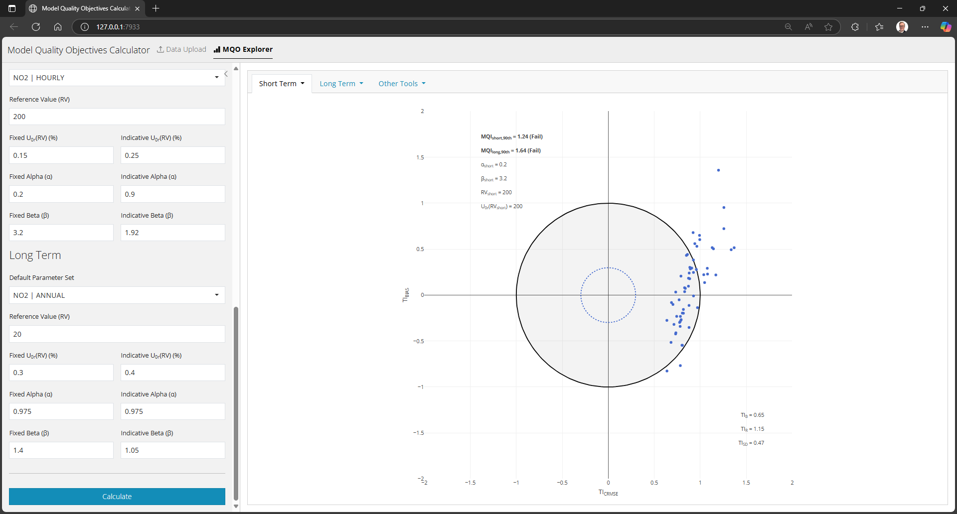
Parameters

For each of the short- and long-term periods, you must provide a parameter set which includes a reference value, a U0(RV) value, and Alpha and Beta parameters. The latter three will take different values for fixed and indicative monitoring. You may choose a ‘Default Parameter Set’ which will automatically fill in these fields with recommended values for different pollutants and statistics.

Outputs

On clicking ‘Calculate’, the right-hand side of the “MQO Explorer” will become populated with content. The different outputs can be navigated using the drop-down menus at the top of the card.

Each of the outputs are described elsewhere on this website. For interpretation, please refer to the CEN specification.

All of the plots can be saved by clicking on the “save” icon at the top right of each figure. Statistical information can be written to a CSV using the “Other Tools > Download Stats” menu, which runs write_mqo_stats() on the currently displayed statistics tables.