Importing Data
data.RmdThere are three methods for importing data for use in mqor.
The mqor recommended data format, originally developed alongside mqor during its inception project.
Input files expected by the DELTA tool. For the monitoring and measurement data, this can either be a CDF or a directory of delimited files (for short-term data) or a single or collection of delimited files (for long-term data). The
startup.iniis also additionally required, formatted as expected by the DELTA tool. No other DELTA config files are required.Any kind of R object which the user can coerce into a
data.frame(ortibble). It is up to the user to ensure that it is
Each of these will be discussed in turn.
Importing {mqor} Data
mqor recommends the following data structure.
For short-term data, please produce a semicolon delimited file with headings “Stat_Code”, “Pollutant”, “Year”, “Month”, “Day”, “Hour”, “Observation” and “Model”. “Stat_Code”, “Pollutant” and “Year” will be used to join this data to the metadata “attribute” file. “Observation” and “Model” should contain the observed and modelled value, respectively.
For daily data, “Hour” can either be omitted or set to
0.
#> [1] "Stat_Code;Pollutant;Year;Month;Day;Observation;Model"
#> [2] "S1;PM10;2025;1;1;24;48"
#> [3] "S1;PM10;2025;1;2;35;47"
#> [4] "S1;PM10;2025;1;3;44;39"
#> [5] "S1;PM10;2025;1;4;38;37"
Long-term data has much the same structure, although naturally omits “Month”, “Day”, and “Hour”.
#> [1] "Stat_Code;Pollutant;Year;Observation;Model"
#> [2] "S1;PM10;2025;34.4;42.6"
#> [3] "S2;PM10;2025;44.4;48.6"
#> [4] "S3;PM10;2025;53.6;59.6"
#> [5] "S4;PM10;2025;44.8;44.8"
Station metadata is stored in an ‘Attributes’ file. The expected names for this file are “Year”, “Frequency”, “Timeseries_Type”, “Stat_Code”, “Stat_Name”, “Stat_Abbreviation”, “Country”, “Region”, “Area”, “Altitude”, “Lon”, “Lat”, “GMTlag”, “Stat_Type”, “Area_Type”, “Siting”, “Pollutant”, “Measurement_Type”, “Unit”, “Model_Application”, “Model_Type”, “Data_Assimilation”, “Model_Resolution”, “Access”, “Source_Obs”, “Source_Model”, “Derived”, “Derived_Identifier”, “Derived_Comment”, and “Time_Series”. Some important columns here include:
“Year”, “Pollutant”, and “Stat_Code”, which are used to combine the AQ data with the attributes.
“Time_Series”, which is also used to join the data and should include the file name of the data where that attribute row’s year/pollutant/station can be found, including the extension (i.e,
myfile.csv, notmyfile).“Measurement_Type”, which should only contain the words “fixed” or “indicative”. These are vital for properly applying the MQO methodology.
“Stat_Name” and “Stat_Abbreviation”, which are mainly useful for labelling plots. “Stat_Abbreviation” is used throughout mqor by default.
Most of the other fields are useful for filtering; e.g., only calculating statistics for certain site types/countries. Columns like ‘Unit’ and ‘GMTlag’ are currently not used by the software; it is up to the user to ensure dates and units are correct before using the mqor package.
#> [1] "Year;Frequency;Timeseries_Type;Stat_Code;Stat_Name;Stat_Abbreviation;Country;Region;Area;Altitude;Lon;Lat;GMTlag;Stat_Type;Area_Type;Siting;Pollutant;Measurement_Type;Unit;Model_Application;Model_Type;Data_Assimilation;Model_Resolution;Access;Source_Obs;Source_Model;Derived;Derived_Identifier;Derived_Comment;Time_Series"
#> [2] "2025;hour;hour;S1;Station 1;S1;ABC;Capital;Central;50.3;0;0;GMT+0;traffic;urban;unknown;PM10;fixed;µg/m3;TESTING;interpolation;Yes;urban;Private;Irceline;Irceline;Yes;;;demo_shortterm.csv"
#> [3] "2025;hour;hour;S2;Station 2;S2;ABC;Capital;Central;50.8;1;0;GMT+0;traffic;urban;unknown;PM10;fixed;µg/m3;TESTING;interpolation;Yes;urban;Private;Irceline;Irceline;Yes;;;demo_shortterm.csv"
It is recommended to read these files using read_mqor().
To demonstrate, we’ll use some in-built CSV files useful for
demonstration.
demo_files()
#> [1] "demo_attributes.csv" "demo_longterm.csv"   "demo_shortterm.csv"
read_mqor() takes two main arguments -
file_data and file_attributes which are paths
to either short- or long-term data, and optionally an attributes file.
read_mqor() can work out whether the data is short- or
long-term by the presence of the "Month" column, so the
user does not need to intervene.
mqor_short <-
  read_mqor(
    file_data = demo_files("demo_shortterm.csv"),
    file_attributes = demo_files("demo_attributes.csv")
  )

mqor_long <-
  read_mqor(
    file_data = demo_files("demo_longterm.csv"),
    file_attributes = demo_files("demo_attributes.csv")
  )
Importing DELTA Data
mqor can ingest data in a format expected by the DELTA tool. You can read about the DELTA tool at https://aqm.jrc.ec.europa.eu/Section/Assessment/Background.
DELTA accepts multiple formats of data, and mqor can cope with all of them - it is just a case of selecting the correct function:
Short-Term:
CDF Files:
read_delta_data_cdf()A directory of CSV files:
read_delta_data_delim()(NB: this function requires a path to a directory, not an individual file or files)
Long-Term:
A single CSV file:
read_delta_yearly_file()A directory of CSV files:
read_delta_yearly_file()
Other Files:
Anything in the ‘resources’ directory:
read_delta_resource()Anything in the ‘config’ directory:
read_delta_config()(NB: mqor doesn’t require anything from the ‘config’ directory)
When importing data, you will have to tell the function whether you
are reading in observations ("obs") or modelled data
("mod") using the data_type argument in almost
all situations. You will also need to read the startup.ini
file from the resources directory. Currently,
mqor has no use for any other DELTA config files. Once
you have monitoring, modelling, and startup data, the
fmt_delta_for_mqor() will assemble them together. As DELTA
has no concept of ‘fixed’ or ‘indicative’ sites, you will need to tell
fmt_delta_for_mqor() how to label the data at this
stage.
An example workflow is outlined below.
# metadata
startup <- read_delta_resource("startup_demo.ini")

# short term
monitoring <- read_delta_data_delim("monitoring", data_type = "obs")

modelling <- read_delta_config("modeling/mymodel.cdf", data_type = "mod")

mqor_short <-
  fmt_delta_for_mqor(monitoring, modelling, startup, data_type = "fixed")

# long term
monitoring_long <- read_delta_yearly_dir("monitoring_annual")

modelling_long <- read_delta_yearly_file(
  "modeling/annualdata.csv",
  data_type = "mod"
)

mqor_long <-
  fmt_delta_for_mqor(
    monitoring_long,
    modelling_long,
    startup,
    data_type = "fixed"
  )
Using Other Data
There is nothing stopping a user using mqor
interactively (i.e., in an R console and not with
launch_app()) from creating an appropriate data object
themselves from any source. mqor follows typical modern R
package design paradigms in working on a single “tidy”
data.frame. In its most simple implementation,
mqor needs six columns:
A numeric column containing observations from air quality monitoring, which defaults to
"obs".A numeric column containing corresponding modelled data, which defaults to
"mod".A character or factor column distinguishing between different sampling points, which defaults to
"site".A character or factor column distinguishing between different pollutants, which defaults to
"pollutant".A character or factor column distinguishing between different measurement types, which defaults to
"type"and can only contain"fixed"or"indicative".A POSIXCt column containing the datetime of the observation/modelled value (short-term) or an integer column containing the year of the values (long-term), which defaults to
"date".
All “metadata” columns like site type, longitude, latitude, and so on aren’t strictly needed in an interactive session; it is up to the user to filter their data however they choose.
Let’s construct an mqor-ready dataset by hand to demonstrate. Long-term data is the easiest to mock up:
set.seed(123)

# invent some random numbers for observed values
obs <- sample(30:50, size = 15, replace = TRUE)

# add some noise for modelled values
mod <- jitter(obs, factor = 10)

# randomly allocate these to fixed/indicative
type <- sample(c("fixed", "indicative"), size = 15, replace = TRUE)

# create data frame
thedata <-
  dplyr::tibble(
    obs = obs,
    mod = mod,
    type = type,
    site = LETTERS[seq_along(obs)], # make up some site codes
    param = "PM10", # assign all to PM10
    date = 2020 # assign all to 202
  )

print(thedata)
#> # A tibble: 15 × 6
#>      obs   mod type       site  param  date
#>    <int> <dbl> <chr>      <chr> <chr> <dbl>
#>  1    44  44.4 indicative A     PM10   2020
#>  2    48  47.2 fixed      B     PM10   2020
#>  3    43  41.6 fixed      C     PM10   2020
#>  4    32  33.9 fixed      D     PM10   2020
#>  5    39  40.6 fixed      E     PM10   2020
#>  6    47  47.8 indicative F     PM10   2020
#>  7    40  41.2 fixed      G     PM10   2020
#>  8    34  32.1 fixed      H     PM10   2020
#>  9    49  48.9 indicative I     PM10   2020
#> 10    43  44.0 fixed      J     PM10   2020
#> 11    34  32.9 fixed      K     PM10   2020
#> 12    48  47.3 fixed      L     PM10   2020
#> 13    38  36.9 fixed      M     PM10   2020
#> 14    32  30.6 indicative N     PM10   2020
#> 15    37  36.7 indicative O     PM10   2020
To prove that this has worked, we can plug our dummy data straight into mqor functions and analyse it.
plot_mqi_scatter(summarise_mqo_stats(thedata, pollutant = "PM10"))
#> ! term assumed to be 'long'.
#> ℹ If this is incorrect, please specify the data's term using the term argument.
#> ! Using fixed long-term annual pm10 parameters.
#> ℹ If this is incorrect, please use `mqor::mqo_params()` or
#>   `mqor::mqo_params_default()` to construct a parameter set.
#> ! Using indicative long-term annual pm10 parameters.
#> ℹ If this is incorrect, please use `mqor::mqo_params()` or
#>   `mqor::mqo_params_default()` to construct a parameter set.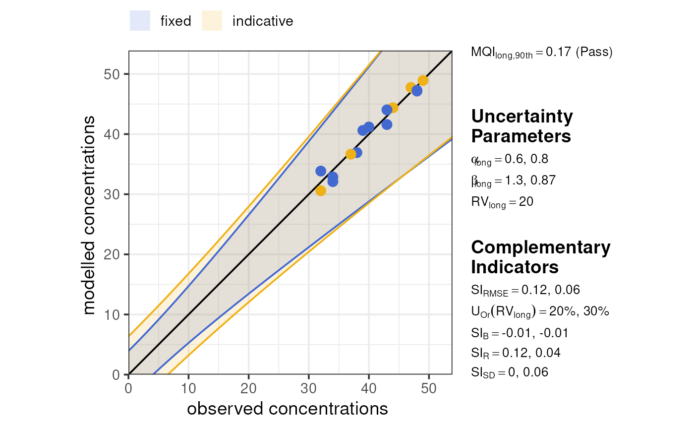
In reality, you are unlikely to create a dummy dataset like this. But you may access data from a database, or download it from the web, or read it from a local file. You should use whatever tools are appropriate to reshape your data into the structure shown above.
For example, the openair package is a common way to obtain UK air quality data. Let’s say we’ve obtained long-term (annual) averages using it.
ukaq_2025 <- openair::importUKAQ(
  source = "aurn",
  year = 2025,
  to_narrow = TRUE,
  pollutant = c("no2"),
  data_type = "annual",
  progress = FALSE
)
There are no “modelled” values here, so let’s pretend the 2024 concentrations are our modelled values. In reality, we may obtain our modelled data from another source.
ukaq_2024 <- openair::importUKAQ(
  source = "aurn",
  year = 2024,
  to_narrow = TRUE,
  pollutant = c("no2"),
  data_type = "annual",
  progress = FALSE
)
We can now join these together in R. We’ll also take the opportunity to tidy them up somewhat, and define the year and monitoring types.
joined <-
  dplyr::left_join(
    ukaq_2025,
    ukaq_2024,
    by = c("source", "code", "site", "species"),
    suffix = c("_obs", "_mod")
  ) |>
  dplyr::select(-dplyr::contains("_capture"), -dplyr::contains("date")) |>
  dplyr::mutate(type = "fixed", year = 2025)

dplyr::glimpse(joined)
#> Rows: 204
#> Columns: 8
#> $ source    <chr> "aurn", "aurn", "aurn", "aurn", "aurn", "aurn", "aurn", "aur…
#> $ code      <chr> "ABD8", "ABD9", "ACTH", "AH", "ARM6", "AYLA", "BAAR", "BALM"…
#> $ site      <chr> "Aberdeen Wellington Road", "Aberdeen Erroll Park", "Auchenc…
#> $ species   <chr> "no2", "no2", "no2", "no2", "no2", "no2", "no2", "no2", "no2…
#> $ value_obs <dbl> 22.077423, 14.605700, NA, 2.969622, 21.239139, NA, 16.531980…
#> $ value_mod <dbl> 24.301062, 13.916347, NA, 2.430615, 21.799815, NA, 14.119127…
#> $ type      <chr> "fixed", "fixed", "fixed", "fixed", "fixed", "fixed", "fixed…
#> $ year      <dbl> 2025, 2025, 2025, 2025, 2025, 2025, 2025, 2025, 2025, 2025, …
When working with data from other sources, if the only difference
between your data and the data above is the column names, you can tell
many mqor functions to remap the columns they expect with
the mqo_dict() function. Let’s use that now to use our
newly imported data.
# define a name dictionary
name_map <-
mqo_dict(
obs = "value_obs",
mod = "value_mod",
type = "type",
site = "site",
pollutant = "species",
date = "year"
)
# use function with dictionary
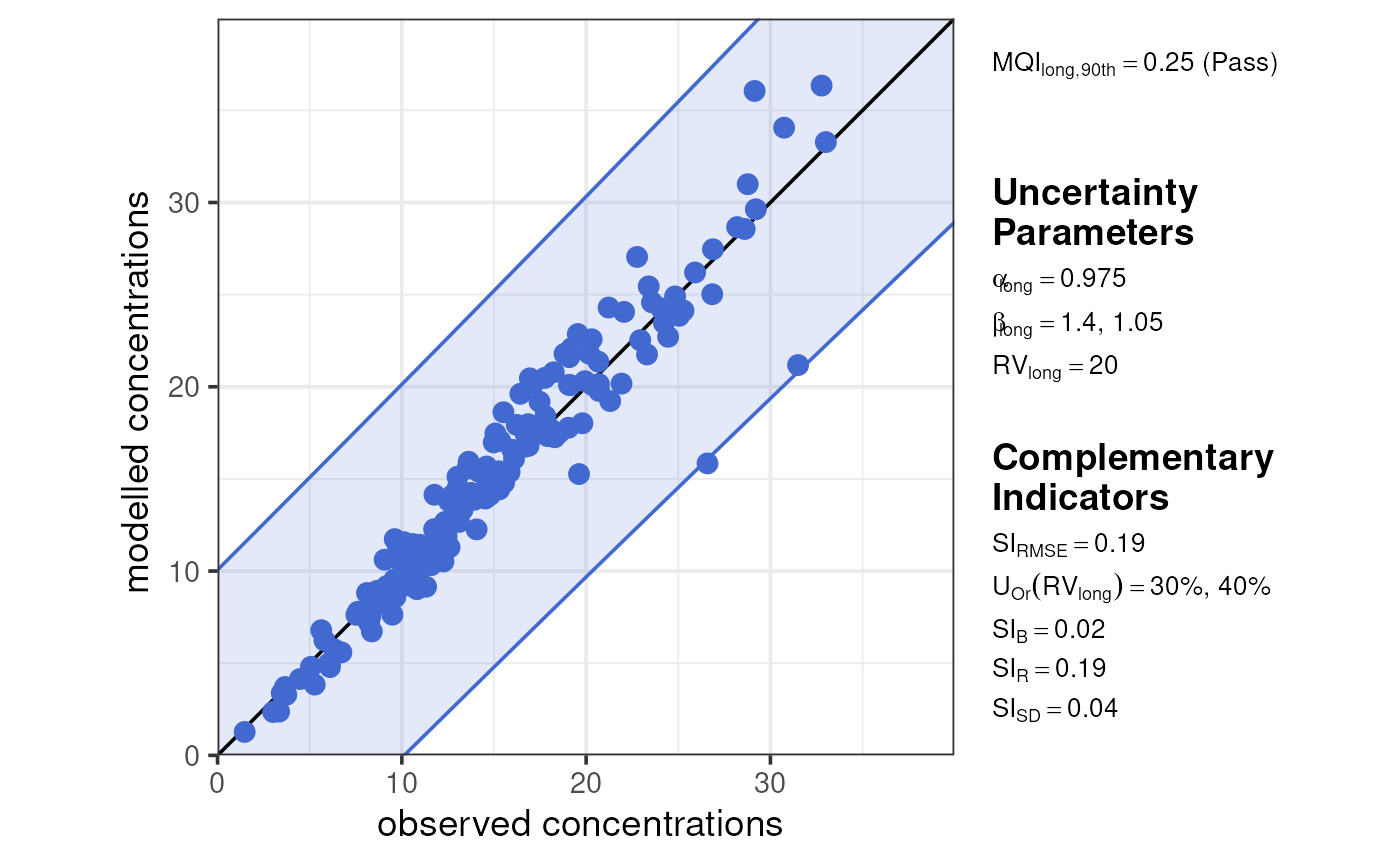
plot_mqi_scatter(summarise_mqo_stats(joined, pollutant = "no2", dict = name_map))
#> ! term assumed to be 'long'.
#> ℹ If this is incorrect, please specify the data's term using the term argument.
#> ! Using fixed long-term annual no2 parameters.
#> ℹ If this is incorrect, please use `mqor::mqo_params()` or
#> `mqor::mqo_params_default()` to construct a parameter set.